Distance Azimuth Surveys

Introduction
The goal of this lab was to get field experience collecting distance data using various instruments. The instruments were used at one starting point to measure the distance and azimuth of ten trees (per instrument) and the diameter of each tree. Some of these instruments were basic instruments so that the field methods class could get comfortable using them. A few maps were made to present the data and to consider the accuracy of the three different distance collecting techniques.

Figure 1. Three different surveys were conducted in Putnam Park, which resides on University of Wisconsin - Eau Claire property.

Study Area
The surveys were conducted in Putnam Park (Figure 1), which is a nature trail on the University of Wisconsin - Eau Claire campus that is often used in scientific exercises. The area of the trail that the surveys were conducted on was dense with trees and it lay at the foot of a tall hill. The challenges associated with this study area were the amount of trees, the cool temperature and the rough, low-lying terrain.

Methods
There were three instruments involved in taking the three surveys. Each survey was taken at a different location in Putnam Park. All the data collected were put into an excel file which included the location of the survey spot (latitude and longitude), distance, azimuth (direction) and diameter of the tree. A GPS unit was used to collect the location of each survey site. A tape measure specially designed with a hook for measuring the diameter of trees was used for every tree. Different tools were used at each site to find the distance and azimuth of each tree. Ten trees were measured at each site.

Survey Site 1:
The first survey site (Figure 2) used a laser distance finder that found distance and azimuth. The instrument (Figure 3) uses a laser that can calculate distance and azimuth when pointed at an object. In this instance it was pointed at ten different trees.

Figure 2. This laser distance finder had many different settings, but the field methods class used it to find distance and azimuth of ten trees.

Figure 3. A Trupulse 360B was used to conduct the first survey.

Survey Site 2:
The second survey site (Figure 4) used the most basic of instruments to measure distance. A tape measure (Figure 5) was used to record the distance to the trees. A specialized compass was used to calculate the azimuth. This compass had a hole through which the user looks through. With a scale inside of the compass, the user used one eye to read the scale and the other to point the compass at the desired tree.

Figure 4. The measuring tape was easy to use, however the compass required better technique to more accurately calculate the azimuth.

Figure 5. This particular group was the hardest working group in the class and stayed longer than any other group in freezing temperatures.

Survey Site 3:

The third survey site (Figure 6)  used a two-piece distance finder (Figure 7) as well as the compass used in the previous survey site. The two-piece distance finder required one scientist to stand in front of the desired tree holding the receiver end of the finder while another scientist stood at the survey spot using the laser piece of the finder. The laser piece of the distance finder calculated the distance. The specialized compass was used to calculate the azimuth again.

Figure 6. The two-piece distance finder was the last instrument used to determine distance.

.

Figure 7. This two-piece distance finder was useful for quick measurements.

Discussion

The laser distance finder seemed to be the easiest tool to use, because it calculated distance and azimuth all at once. This saved a lot of time. The next easiest tool to use was the two-piece distance finder, however the accuracy was skewed because the target was not the actually tree, but the person standing in front of the tree. Also, the compass used to calculate azimuth was very tough to use, because it required the user to use each eye to see different things at one time. The measuring tape was the most time consuming tool to use, because the terrain was full of brush and the measuring tape would get stuck on sticks and bushes.

Overall, I believe that the laser distance finder was the most accurate because it measured distance to the actual tree. The other two surveys needed to use the compass, which I believe wasn't as accurate because it was tough for the user to use. The distance for the two-piece distance finder was not as accurate because the user needed to stand in front or next to the tree, so the distance was never exact. The tape measure had to wind around other trees and brush which affected the distance.

A few problems occurred in the collection and mapping of the data. The group had to record an extra 10 distances of trees due to a lack of organization during the data collection. This costed the group an extra 10 minutes of time. When mapping the data, the latitude and longitude of survey site one was incorrect, so I had to estimate the location of the site on the imagery base map and determine the latitude and longitude from that spot.

Processing Phantom 3 Drone Data

Introduction
The goal of this lab was to become familiar with unmanned aerial vehicle (UAV) data. UAVs are becoming more applicable in many different scientific fields, therefor it is an important to become acquainted with this technology. The data used in this lab was collected by Dr. Joe Hupy (University of Wisconsin - Eau Claire) using a Phantom 3 drone.

Methods
The Phantom 3 drone was flown at a height of 60 meters. The data was processed using Pix4D software. Once creating the file in the software, the images were added to the file, including the metadata associated with the images. Next, the software assumed that the camera used on the UAV was a global shutter, which was wrong, so it was changed to a Linear Rolling Shutter. The software gathered the coordinate system for the system from the metadata. Once the settings were correct the program showed the overall layout of the flight. At this point initial processing could begin. Initial processing lasted a few minutes. Once it finished, the point cloud and mesh along with the digital surface model, orthomosaic image and index were generated. These last two steps lasted about 15 minutes. Data quality reports were created after each of the 3 processing steps were finished. The final product was two maps created using the processed data in ArcMap.

Results
Two maps were produced using the UAV data; a DSM (figure 1) and a mosaic image (figure 2).

Figure 1. A DSM model was produced using the UAV data. One meter contours were added to accent the changes in elevation.

Figure 2. A mosaic image was created to display the effectiveness of the Pix4D software in generating mosaic images.

Reaction

Pix4D was very user-friendly, meaning that it was not a complex software to use. It generated images that can be used for a variety of purposes. Some of the defaults were too presumptive though, and one must be careful to check all the defaults in the program.

Survey 123: A tutorial

Introduction
The main objective of this lab was to become acquainted with Esri's Survey123, which is an application that works with ArcMap and ArcMapOnline to create surveys. These surveys can be extremely helpful in collecting geospatial information without having to go out into the field. The idea is that willing participants fill out the survey supplying the desired information, including a location, if need be. In this lab the tutorial Get Started with Survey 123 for ArcGIS provided by Esri Online was taken. This tutorial includes four lessons.

Lessons
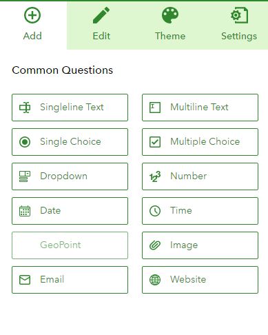
The first lesson demonstrated how to create the survey. After logging into the UWEC enterprise account for Esri a new survey was created, which involved adding different kinds of questions (Figure 1). In the tutorial a HOA Emergency Preparedness survey was created using 28 questions related to preparedness in the case of a disaster.

Figure 1. Survey 123 provides multiple types of questions to be added to the survey.

The second lesson showed how to make the survey available to other people. In this instance the survey was made available to only those in the UWEC enterprise account. The survey can be accessed by a URL. The tutorial called for the survey to be completed eight times. I made sure to vary the answers submitted to get more interesting results. This section also revealed that Esri created a Survey123 app so that surveys could be taken with a smartphone (Figure 2).

Figure 2. This is a screenshot of the Survey123 app on an iPhone 6.

The third lesson explored the analyze and data tab, where data from the survey can be viewed in different charts and tables. All of the data collected from the survey was arranged in many different tables that were easy to read and use. This information is useful when writing reports about the collected data. Especially useful for the geospatial aspect of ArcGIS is the use of a map that displays where the survey-takers' homes were (Figure 3).

Figure 3. Spatial information of the survey-takers' homes were provided by the survey-takers.

The last lesson demonstrated how to share display the map in ArcGIS Viewer and how to share that map. The user could manipulate map colors and the way the spatial data is displayed (Figure 4). Everything from Pop-ups to the data point could be manipulated. The map can then be shared as a web map for the rest the public (or university enterprise account) to see.

Figure 4. The web map shows geospatial data collected from the survey.

Results & Conclusion

The results of the map are random. When filling out the survey I tried to answer the questions based on where the "survey-taker's" home was. While filling out the survey, sometimes I claimed to have a house in areas where disasters occured more often. Unfortunately, I mentioned a state or city rather than a specific address, so the survey assumed the house was in Eau Claire, WI (where the survey was taken).

Survey123 can be extremely useful in fields where specific information about people are needed with geospatial information. My field of study does not involve information by a broad range of people, so this survey does not suite my study needs, but I still think that it could be extremely useful in other science fields.

Lab 6: Creation of a Navigation Map

Introduction
Tools and a location system are key in the process of navigation. Tools could be anything from the stars in the night time sky to an expensive GPS unit. A location system is important in finding out where you are during navigation. A location (coordinate) system can use latitude and longitude or other forms of geographic scales, depending on the scale of navigation. Different coordinate systems are used depending on the study area to provide better accuracy in determining a location. The purpose of this lab is to create two navigation maps using two different coordinate grids.

Study Area
The Priory is a dormitory belonging to the University of Wisconsin - Eau Claire. This dorm is nestled in a wooded area located roughly 2.25 miles SSW of the University (Figure 1).

Figure 1. The priory is about a 10 minute drive from the university.

Methods
Two maps were created in ArcMap with each using different coordinate systems. They share the same 3 meter contours and base map. One map was created using a Universal Transverse Mercator (UTM) Coordinate System and the other uses a Geographic Coordinate System (GCS). The data can be found in the class share folder in the Priory geodatabase.

UTM
This coordinate system divides the globe into 60 north and south zones. Each zone has its own central meridean with the equator dividing the north and south zones (Figure 2).

Figure 2. This image shows the UTM zones found in the United States. Image from Wikipedia.

GCS
This coordinate system uses latitude and longitude in decimal degrees(Figure 3). While the UTM uses the transverse mercator the GCS is not attached to any particular projection.

Figure 3. The distance represented by one degree of longitude decreases as the meridians converge at the North and South Poles. Image provided by ArcMap Desktop Web Help.

Results
The first map (Figure 4) uses the WGS 1984 UTM Zone 15 N projected coordinate system. The second map (Figure 5) uses the WGS 1984 geographic coordinate system. The geographic coordinate system produces more distortion in the image, so it would be better suited for navigation.

Figure 4. This map grid uses 50 meter spacing.

Figure 5. This map grid is in decimal degrees.

Conclusion
This lab showed that creating a navigation map requires a more practical map setup. This set up must be easy to read so that the user can navigate using this along with a basic compass. Navigation maps are important in times when technology such as GPS aren't an option. The grid and elevation contours are added to help users visualize the landscape. The UTM grid will prove most useful in the next lab.

Lab 5: Visualizing the Terrain Survey

Introduction

In the previous lab (#4), a four square foot sandbox was used to create a strategic terrain from which elevation data could be collected to create digital models.

Figure 1. Normalized data table.

The purpose of this lab was to create the digital models using elevation data gathered from the previous lab. It is important to consider data normalization when collecting samples in geospatial surveys. Data normalization is the "cleaning up" and organizing of data into columns or tables to improve data integrity. In this case, the data collected in Lab 4 was put into an Excel spreadsheet (Figure 1), because it was compatible with the GIS programs that were used later, ArcMap and ArcScene.

The samples in lab 4 were collected using a grid with 6 cm intervals and a sample was collected at every grid intersect (Figure 2). These samples points were plotted in ArcMap and interpolated to create a 3D model in ArcScene. This lab will examine the effectiveness of the data collection method in its ability to create an accurate digital terrain model using 5 interpolation methods.

Figure 2. Sandbox with terrain and grid.

Methods

Once the data points were imported into ArcMap, interpolation was used to visualize the terrain model. According to ArcHelp, interpolation is used to create a continuous surface from the provided sample point values. Here are the 5 interpolation techniques used in this lab as described by ArcHelp:

1. Inverse Distance Weighted (IDW)-Determines cell values using a linearly weighted combination of a set of sample points.

Advantages: Can set parameters to how heavily the control point is weighted.

Disadvantages: Unevenly spaced data points will result in an unrealistic model.

2. Natural Neighbor-Uses an algorithm that finds the closest subset of input samples to a query point and applies weights to them based on proportionate areas to interpolate a value.

Advantages: It creates a smooth surface, even if data is missing.

Disadvantages: Has a limit of about 15 million input points.

3. Kriging-An advanced geostatistical procedure hat generates an estimated surface from a scattered set of points with z-values.

Advantages: Predicts empty spaces by analyzing spatial behavior derived from z-points, which can create extremely accurate 3D models.

Disadvantages: Can create a highly inaccurate 3D model when not enough data points are present.

4. Spline-Uses a mathematical function to estimate values and minimize overall surface curvature.

Advantages: Results in the smoothest surface of all the other interpolation techniques.

Disadvantages: Can be produce an inaccurate 3D model if the original terrain is not smooth.

5. Triangular Irregular Network (TIN)-Constructs a vector surface made up of triangles by triangulating a set of vertices.

Advantages: Can have a higher resolution in areas where a surface is highly variable.

Disadvantages: The hard-line edges of each triangle are highly unrealistic to any sort of terrain in nature.

In ArcScene the 3D models were exported as JPEGs. 

Results/Discussion

Below are the images of all the 3D models created using the 5 interpolation methods. Since letters were incorporated in the terrain a head-on orientation was used to read the "hidden message". The models were also tilted slightly to show how dynamic the terrain features are.

IDW:

This interpolation method did well in pronouncing the sharp edges of our desired letters. However, the many peaks that result from this method are unrealistic and unattractive.

Figure 3. IDW model

Natural Neighbor:

This method proved to be very accurate, however some random points in the plains areas are too pronounced. This model looks more realistic than the IDW method.

Figure 4. Natural Neighbor model

Kriging:

This method represented the sandbox terrain the worst. It showed hardly any change in elevation and lacked any sharp edges that were present in the sandbox. This may have occurred due to the sharp edged of the terrain and inefficient amount of data points.

Figure 5. Kriging model

Spline:

This method captured the terrain of the sandbox the best. It captures the dynamic change in elevations of the letters while still keep a smooth, realistic surface.

Figure 6. Spline model

TIN:

This model does a great job of capturing elevation. However, the smooth plain looks rougher than it should and the blocky nature of the TIN model creates an unrealistic texture.

Figure 7. TIN model

The 6 cm interval grid proved effective in the number of data points collected in most interpolation models. The only model that had absolutely no resemblance to the sandbox terrain was the kriging model. However, the terrain that was meant to represent a "heart" did not show up in any model as effectively as the other letters. This may be due to the combination of curve and change in elevation occurring at the two upper "humps" of the heart. Such a drastic curve is tough to capture through a grid set-up.

Conclusion

Using a 4 by 4 foot sandbox, a dynamic terrain was created and a systematic grid survey technique was used to capture elevation. Once the elevation data was normalized, it was imported into ArcMap and ArcScene to use various interpolation methods to observe which interpolation method created the most realistic 3D model. This survey technique is comparable to any other survey technique that collects elevation data, either large-scale or small-scale. One of the most important of those survey techniques that is similar to this lab is LiDAR, which uses millions of data points to create terrain models. This difference with this lab is that very basic equipment and techniques were used to collect the data and this survey was at an extremely small scale. The grid based survey is not always necessary, especially when the study area is large. It would be quite difficult to set up a grid when there are objects in the way of intersections and grid lines.

Lab 4: Creation of a Digital Elevation Surface

Lab 4: Creation of a Digital Elevation Surface

Introduction
The objective of this lab was to construct an elevation surface, survey the terrain and record the elevation of it using a proper coordinate system and survey technique. Students worked in groups of three to construct a diverse terrain using a 4 square foot sandbox. Group 3 decided to carry out this exercise on Friday, January 27th at approximately 11:00 AM. Group 3 considered a variety of sampling techniques before beginning the outdoor portion of the exercise. Sampling is a method used to gather data on an entire population by collecting data on a smaller, yet representative portion of that population (Royal Geographical Society). This method can be quick and cost-effective when collecting spatial data, especially when a large study area is involved. There are three main types of sampling:

• Random-sample points are chosen at random
• Systematic-samples that are distributed evenly in a spatial context
• Stratified-samples that are taken in sub-sets to more accurately represent different portions of the whole population

Methods

Materials used for lab:

• Sand
• Meter stick
• Thumb tacks
• String
• Notebook
• Spoon (to carve out terrain)
• Measuring tape

Group 3 determined that systematic sampling would be the most appropriate sampling technique for this lab. By using a simple coordinate system and collecting samples at each X,Y intersection it would be simple to record the data in a table. It would be difficult to keep track of and plot data collection points on a table using random and stratified sampling techniques.

After some consideration, Group 3 decided that the coordinate system grid would contain 6 cm intervals in order to collect an effective amount of sample points while being time-effective. Zero elevation was determined to be the top of the wooden frame. A meter stick was used to measure elevation.

The outdoor portion of this activity was conducted under cold and snowy conditions and, while the team was dressed appropriately, the weather conditions played a factor in the speed at which the data was collected. The work was split up evenly. Max and Shannon began to carve out the terrain using their hands and a spoon while Alex placed thumb tacks at 6 cm intervals starting from the inner edge of the wooden sandbox resulting in the use of 19 thumb tacks on each side of the sandbox (Figure 1). The terrain was constructed to contain a hill, ridge, valley, depression and a plain. Next, Shannon and Max worked together to carefully lay the grid by wrapping string around the thumb tacks set up by Alex (Figure 2). Once the grid was set up data was collected at every intersection starting at the determined 0,0 grid point. Alex held the yard stick at every intersection while Max read the measurement to Shannon so she could record the measurement in a notebook. The collected data could not be directly entered by computer because the weather proved harmful for a computer, so the data would later be transfer to an Excel spreadsheet. Setting up the grid and collecting the samples took about 2 hours to complete. 

Figure 1. Max and Shannon created a unique terrain while Alex (taking picture) placed thumb tacks.

Figure 2. Max and Shannon lay out a grid using string.

Results

401 elevation sample points were collected and entered into an Excel spreadsheet (figure 3). Here is some sample values:

Figure 3. Column Z contains elevation data. Values
are negative since samples were collected below "sea level".

• Minimum:-0.8 cm
• Maximum:-11.0 cm
• Mean:-5.2 cm
• Standard Deviation:2.0 cm

The systematic sampling method worked very well. Group 3 stuck with the systematic sampling method for the entire exercise, although there were some concerns of whether the more drastic changes in terrain were captured thoroughly with the amount of samples taken or not. 

Some problems that were encountered during data collection included the shifting of the sand. When the meter stick would contact the sand, the sand would sometimes crumble and change the initial elevation of the model. Human error could have also played a role in collecting data. In order to read the meter stick Max had to get to "sea level", which required him to bend over and some error in reading the meter stick could have occurred after some fatigue.

Conclusion

This exercise appropriately fits the definition of sampling when it comes to collecting data spatially. Unless a mold of the elevation terrain was created, there is no exact way of creating a model of an area. Sampling gives a geographer the ability to create a model that can be as accurate as necessary for the geographer's use without spending a ridiculous amount of time and energy creating an exact model. An advantage of sampling is that it can be used at any scale, from an area as small as a sandbox (Figure 4.) to an area as large as a forest. Sampling can be used to collect data over larger areas as well. 

Figure 4. The unique terrain spells out "I love EC".

This survey did perform an adequate job of sampling the sandbox, however some improvements could be made. Time-permitting, the grid intervals could be decreased to about 4 or 5 cm to create more samples so that the more dynamic terrain could be better represented in the model. Also, stratified sampling could be used to collect more samples of the dynamic terrain that was isolated into sub-sets.

Sources

Royal Geographical Society. Retrieved January 29th, 2016

from http://www.rgs.org/OurWork/Schools/Fieldwork+and+local+learning/Fieldwork+techniques/Sampling+techniques.htm.